The Wagner Projections (Part 3): Umbeziffern – The Wagner Transformation Method
Part 3 of this article series was supposed to be about the Wagner variants created by Frank Canters and Dr. Rolf Böhm. For a better comprehension of these variants it occured to me that before that, it might be better to explain the method that Wagner used to create his nine projections: Das Umbeziffern – a term which might be translated as »renumbering« or »coordinate transformation« or maybe »re-assigning of values«. In this article however, I’ll just stick to the german word.
Karlheinz Wagner particularised Umbeziffern in 1949 [1], Frank Canters provided a nice summary [2]:
The transformation method is based on a very simple idea, but provides a powerful mechanism for the development of new map projections. First a well-chosen part of the graticule of an existing projection, bounded by an upper an a lower parallel, and a left and right meridian, is selected. The entire area to be represented is mapped onto this part of the graticule by redefinition of the longitude and latitude values of each meridian and parallel (Umbeziffern). Then the graticule is enlarged to the original scale of the parent projection. Restoration of the original scale may be followed by an affine transformation in the x- and y-direction. This permits control of the ratio of the axes of the projection.
Let’s illustrate the transformation method using the construction of Wagner VII as example.
Umbeziffern, step by step
As parent projection, Wagner chose the equatorial aspect of the azimuthal equal-area projection; using the part between 65° N/S and 60° E/W for the new projection.

The area to be represented – in this case, it’s the entire earth – is mapped onto this part, then the graticule is enlarged to the original scale of the parent projection:

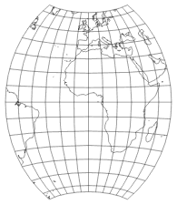
By an affine transformation, we control the ratio of the axes. The equivalence of the parent projection is preserved. The Wagner VII projection is complete:

So up to this point, the new projection is determined by the following parameters:
- The parent projection;
- the bounding parallel;
- the bounding meridian;
- and the scaling factor to control the ratio of the axes.
Within this article, we’ll confine ourselves to Wagner VII and VIII, which both are based on the equatorial azimuthal equal-area projection. So we’ll drop parameter #1 and take it as a permanent feature. That’ll leave us, for the moment, with three parameters.
Before continuing, I’d like to point out that the chosen bounding parallel in effect determines the length of the pole line of our new projection, while the bounding meridian determines the curvature of the parallels. To clarify, let’s look again at the part of the parent projection, but this time bounded by 80° North/South, and bounded by 90° East/West:


Parent projection truncated at 80° N/S and 60° E/W (left);
truncated at 65° N/S, 90° E/W (right).
It’s quite obvious that higher degree values of the bounding parallel will result in a shorter pole line of the new projection, and higher degree values of the bounding meridian will result in a stronger curvature of the parallels.
Let’s go on:
As I’ve said, Wagner VII is an equal-area projection, just like its parent projection. So Wagner added
two further parameters to control areal distortion:
Man kann nun vorschreiben, dass beim Parallelkreis φ1 die Flächenverzerrung nicht größer als S1 sein soll (…)
You can prescribe that at the parallel φ1 the areal distortion should not exceed S1 (…)
For the projection nowadays known as Wagner VIII, Wagner set φ1 = 60 and S1 = 1.2, i.e. an areal inflation of 20% at 60° N/S. These values were chosen because between ± 60° »you roughly get the populated parts of the earth« and »an areal inflation of 20% for the specified area still seems sustainable«.
So the final list now contains five configuration parameters – and this time, we add the notations usually used in cartographic literature:
- The bounding parallel: ψ1
- The bounding meridian: λ1
- The reference latitude for the areal distortion: φ1
- The amount of areal inflation at φ1: S1
- The axial ratio: p
And now, you’re surely beginning to guess what Messrs. Canters and Böhm did to build their Wagner variants: Correct,
they started to twiddle with exactly these five parameters. I’m going to review their result in the
pending fourth fifth part
of the article series.
But before that, I’ve still got to mention a thing or two…
Notation
In cartographic literature, you’ll often find the term Wagner constants (or something like that) – because the formulae that Wagner used for his projection, contain a few numerical values, like for Wagner VIII:
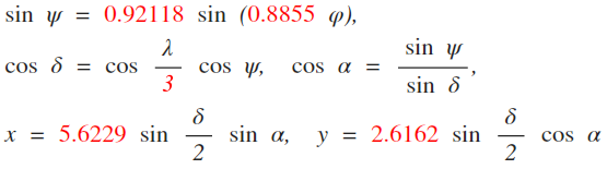
I’ve highlighted the constants I’m talking about using red print.
But how did Wagner come up with exactly these numerical values?
Well, he used his five input parameters mentioned above, processed them through a bunch of
formulae, and ended up with some numerical values, that he inserted in the final formula for
convenience of the reader. Of course, with these numerical values you can only
generate Wagner VIII. But instead, you could also write a generalized version of the formula:
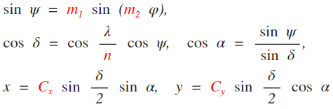
Now, you just have to insert appropriate values for m1, m2, Cx, Cy and n – and you’ll have a Wagner variant, just like those presented by Canters and Böhm. So how do you get some »appropriate values«? – You can calculate them from the five configuration parameters mentioned above, like e.g. Dr. Böhm showed in his paper. That document is in german, however if you read formulae 7 to 12 on page 4/5, I think you’ll get the idea even if you don’t understand German.
And there’s another way to get the values.
But hang on a bit, I’ll come back to that in a moment.
Before that, I’d like to mention that Dr. Böhm proposed a very convenient notation to identify Wagner variations:
A simple list of the 5 convenient parameters, separated by a dash. The first three parameters are written
in their usual values in degree. For #4 and #5 he decided to use percental values, so that an areal inflation
of 1.2 is written as 20, and if the equator shall be twice as long as the central meridian,
it is noted with 200.
Thus, Dr. Böhm’s notation for Wagner VII is 65-60-60-0-200 and for Wagner VIII, 65-60-60-20-200.
I think that’s a great idea, because for one thing the values are easier to memorize than the constants (0.92118 etc). But mainly because the values are directly tied to the parent projection, and if you keep the step-by-step images shown above in mind, you might be able to picture (at least approximately) a configuration like e.g. 65-84-60-25-200, even before you have actually seen it.
However, there’s a little catch: Different notations might result in identical projections. So this notation is unique but not bijective, i.e. there’s no one-to-one relation between the noted values and the actual projection. For example: As I’ve said before, Wagner VIII shows an areal inflation of 1.2 at 60°. That corresponds to 1.89 at 80°, so instead of writing 65-60-60-20-200, you could also write 65-60-80-89-200. One could avoid that by agreeing to always note the areal distortion at 60° – so Wagner VIII would be 65-60-20-200 – or the other way round, to always note the latitude at which the areal distortion is exactly 1.2 (65-60-60-200).
Dr. Böhm did point this out in his paper, but decided to maintain all five parameters, for reasons of clarity and comprehensibility. I agree with this decision but I strongly suggest that whoever may adopt this notation should always use 60 for the third parameter.
Remark:
I would have preferred to write parameters #4 and #5 as factor instead of percent.
In that case, Wagner VIII would be 65-60-60-1.2-2, not 65-60-60-20-200. The reason’s quite simple:
20% feel, for me, like a deflation. Of course, I get that it’s an inflation by 20%
of the original value and it’s not scaled-down to 20%. But I think that the factor would’ve been
more comprehensible.
Nonetheless, I stick to the notation as it was proposed by Dr. Böhm. After all, he is the
map projection professional, not me. It was introduced in a cartographic specialist magazine, it would’ve
felt presumptuous to claim that I know it better…
… what about the other Wagner projections?
Now, I have explained the method of Umbeziffern by the example of Wagner VII, and how to derive the Wagner VIII. Since Wagner used Umbeziffern on all the projections that are named after him, you can modify them in the same way, but there are fewer options:
- On all nine projections, you can modify the length of the pole line and the axial ratio – for the pseudocylindricals, the latter one is in effect equivalent to setting the standard parallel.
- Wagner I to Wagner VI are created from pseudocylindric parent projections, thus they’ll always have straight parallels – there’s no parameter that determines the curvature of the parallels.
- Moreover, Wagner III and Wagner VI have equally spaced parallels, hence the parameter changing the areal inflation is dismissed.
- Wagner IX, too, has equally spaced parallels (along the central meridian) so the areal inflation isn’t variable. But at least the curvature of the parallels can be modified, so in my opinion it’s the second most interesting Wagner projection to play with.
As a consequence, I hereby propose a little extension of the Böhm notation:
To clarify which Wagner projection you’re modifying, prefix its roman numerals in
lowercase letters, followed by the @ character.
For example, a variation of Wagner VII would be written as
Wagner vii@65-84-60-25-200,
while a derivation of Wagner IX might be
Wagner ix@67-87-200-82.
I prefer the lowercase letters on the roman numerals to hint at the fact that you’re not talking
about one of the variants that Wagner himself presented.
And keep in mind that Wagner II, V and VIII are variants of Wagner I, IV and VII respectively,
thus you should never use the prefixes ii@, v@ and viii@
but the preceding numeral instead.
Granted, it is kind of … peculiar to propose an extension of a notation that to my knowledge has never been used anywhere except by Dr. Böhm and myself. But at least now you know what I mean when I’ll use that notation…
Render your own Wagner variations – The WVG
I hope that you’re now curios to get to know how this Wagner variations might look. Because I might have just the right thing for you:
The Wagner Variations Generator (WVG).
There, you can modify the configuration parameters, hit the »Render my projection« button, and an image of
the resulting projection will be shown.
It’s available in two flavors:
The WVG-7 modifies Wagners VII (and thus, see above, Wagners VIII);
the WVG-9 is based on Wagner IX.
Apart from entering some values, you can select a predefined projection which can be rendered using Wagner’s formula, so you can select one of them as a starting point for your own experiments.
Furthermore, there are some image options which don’t refer to the projection in itself but the generated image:
You can choose how the continents are displayed (as a grey silhouette, as outlines, with colored countries, or not at all),
the step range of the graticule and the size of the image. To compare your new projection to existing ones,
you can set a background image showing one of the cylindrical, pseudocylindrical und lenticular projections that
are offered here on this website.
You can download the resulting projection as SVG file.
But what am I talking about?
Head over to the Wagner Variations Generator 7
or Wagner Variations Generator 9
and see for yourself…
In case you’re wondering why on the WVG-7 you can modify only four of five parameters and not all of them:
Since I suggested that the reference latitude for the areal inflation φ1 should always be 60°, I felt
it’s appropriate to stick to that value. Moreover, it helps to avoid errors: With φ1 = 60 the
maximum value for areal inflation is 99.999%. Value above that won’t generate an projection image (because an arccos(x) function
will be fed with an illegal value). With φ1 = 80 however, the maximum value is 475.877.
Every specific value of φ1 leads to a different maximum of S1,
but as a result, you’ll always get the same projection.
So in order to avoid the frustrating situation to enter values that can’t generate a projection, I fixated the 60 for the latitude and set
the max. value of distortion to 99.999.
A few more words…
Wagner’s Umbeziffern is a powerful tool to create projections according to your needs and preferences, yet it has its limits: You’ll never be able to escape the general characteristics of the parent powerful. For example, you can’t change the spacing of the meridians, nor will you ever generate such curve shapes as you can using Hufnagel’s system (see corresponding article or the interactive Hufnagel tool on mapthematics.com).
And in case you don’t just wanna play around but create real maps:
Starting with version 3.2, the map projection software Geocart
supports the generalized Wagner, which allows to modify the Wagner VII just like I’ve explained
in this article. It won’t use the Böhm notation, though. But fear not: The WVG-7 will convert the Böhm notation
to the parameter values you’ll have to enter in Geocart.
And by the way…
did I invite you to check out the WVG-7 and WVG-9? ;-)
References
-
↑
Wagner, Karlheinz:
Kartographische Netzentwürfe.
Leipzig 1949. -
↑
Canters, Frank:
Small-scale Map Projection Design.
London & New York 2002. -
↑
Dr. Rolf Böhm:
Variationen von Weltkartennetzen der Wagner-Hammer-Aitoff-Entwurfsfamilie
First publication in: Kartographische Nachrichten Nr. 1/2006. Kirschbaum: Bonn-Bad Godesberg.
Quoted from www.boehmwanderkarten.de/archiv/pdf/boehm_kn_2_2006_2015_complete.pdf (german)
Back to Selected Projections • The Wagner Projections (Part 2) • Part 4 • Go to top
Comments
3 comments
Bojč
Article and demo about Umbeziffern:
http://cartography.oregonstate…
http://cartography.oregonstate…
Peter Denner
There does, however, seem to be a problem with your WVG-9. When a=100, I'd expect the axial ratio of the projection to always be equal to p/100, but this is only the case when p=200. The easiest way to see this is to set psi1=90, lambda1=90, p=100, a=100. I'd expect this to produce a projection with a circular boundary, as the WVG-7 does with these values, but instead it's elliptical with an axial ratio of sqrt(2). This is the value of Cx, and it seems that the axial ratio is always equal to Cx rather than p.
How are p and Cx supposed to be related? I can't see p in the equations above, and the only equation with p that I can see in Dr Böhm's article is equation 10, but this seems to be specific to Wagner VII/VIII:
With the Wagner VII/VIII transformation, you have the two sines in Dr Böhm's equation 3, and with the equal-area azimuthal as the parent projection, I think that the axial ratio before any re-scaling (i.e. if you stop just before "then the graticule is enlarged to the original scale of the parent projection" in your explanation above) should be tan(lambda1/2)/tan(psi1/2), hence all the sines and cosines in equations 7-16. On the other hand, with the Wagner IX transformation, m1=0, so the sines drop out of equation 3, and with the equidistant azimuthal as the parent projection, the axial ratio before any re-scaling should simply be lambda1/psi1, so I wouldn't expect to see all those sines and cosines.
If you let me know what equations you're using for your WVG-9, then maybe I can help spot where the problem lies.
Tobias Jung
thanks for your comment!
First of all, let me say that I’m really not good at math, so it’s always possible that I did some mistakes in transcribing the formula.
Regarding the axial ratio: Yes, this is very confusing, because both p and a change it. When Wagner presented the formula in his 1949 textbook, he started out with assuming an axial ratio of 1:2, i.e. with p = 2. (Sidenote: Instead of 2 I’m using 200 just in order to keep it consistent with Dr. Böhm’s notation).
Then, he develops the final formula over several steps and ends up with the projection that is called "Wagner IX" in the WVG-9.
And THEN, he says: "In order to get the shape closer to the Winkel Tripel (Bartholomew), you can multiply all the x-values with a = 0.88".
That’s the projection I called "Wagner IX.i".
So, why did he do that instead of going back to the fist steps to set p to an appropriate value? My guess is that, back in those days when they didn’t have computers, it was just a whole lot easier to multiply all the x-values than to calculate all the intermediate steps again with a different p.
Later, when Canters developed his optimized Wagner IX, he did the same thing: He left p = 2 and set a = 0.8211.
Looking back, I should have done the same thing: Leaving p = 2 hardcoded in the formula, and just varying the a.
I’m currently writing a proper d3 implementation for the customizable Wagner IX in which I’m doing exactly that. In that version, you actually do get a circular projection when you set psi1=90, lambda1=90, a=100.
As for all those sines and cosines: I actually don’t know why they are all there. Did I mention I’m bad at math? ;-)
I merely transcribed Gerald I. Evenden’s Wagner IX implementation to JavaScript syntax. And they are also there in Wagner’s original text, see:
https://map-projections.net/do…
I hope this answers your questions – if not, feel free to ask again!
Kind regards,
Tobias
Peter Denner
I understand your reasons for including both a and p. While it is a bit confusing, my issue wasn't with the presence of two re-scaling factors but with the fact that any value of p other than 200 produces an incorrect projection. As I've explained below, this seems to come from having Cy=1/m instead of Cy=1/(k*sqrt(m*n)). It just so happens that if p=200, then the equation for Cy simplifies to Cy=1/m, so it works for that value and is close enough that you might not notice the difference for, say, 150
Peter Denner
... you might not notice the difference for, say, 150
Peter Denner
... you might not notice the difference for, say, values of p between 150 and 250.
If you're only going to vary one value and leave the other hardcoded in the formula, then I would leave a hardcoded and vary p, for a few reasons:
Easier comparison with Wagner VII/VIII, where you have p but not a.
The axial ratio p seems a more intuitive input for the user than "the factor that I have to compress the projection by so that I get the axial ratio that I want".
If the equations are sorted such that p does what it's supposed to do, then varying p alters the axial ratio in such a way that the product of the lengths of the axes is unchanged, hence the area is only changed slightly. On the other hand, varying a alters the length of the x axis but leaves the length of the y axis unchanged, so the area can be changed significantly. Some measures of areal distortion are affected by changing the size of the projection even if the shape is unchanged, so varying a messes up quantifying areal distortion. This effect is shown in this thread:
https://mapthematics.com/forum…
Tobias Jung
Regarding the area preservation: It’s not the intention of the renumbering of the Wagner IX to preserve areas – the intention is to create a projection with equally spaced parallels along the central meridian. That’s what Wagner did on all his nine projections:
Wagner I, IV, VII – equal area
Wagner II, V, VIII – compromise projections with "controlled areal inflation"
Wagner III, VI, IX – equally spaced parallels.
Correct me if I’m wrong here (you know, bad at math etc.) but if the demand is to keep the equally spaced parallels AND to keep areal inflation (mostly) as it is, you’d again have to change the pole line length accordingly, thus messing up the value that’s given by the user input.
btw, sometime soon I’ll have to look into that "less than" symbol problem… didn’t notice that before, thanks for spotting it!
Peter Denner
Imagine the axes define a rectangle. Regardless of whether you vary a or vary p, when you alter the axial ratio, you'll also alter the aspect ratio of that rectangle. If you vary a, then you only alter the length of the x axis, not the y axis, so you'll also alter the area of that rectangle. On the other hand, if you vary p, then however much you compress the x axis, the y axis will extend such that the area of that rectangle is unchanged. You can end up with two projections that have exactly the same shape, but depending on whether you've varied a or varied p, the size of the two projections will be different relative to the nominal scale.
Now imagine that rectangle is divided into millions of tiny rectangles, each with the same aspect ratio as the large rectangle. Again, if you vary a, then you'll also alter the area of each of these tiny rectangles. In the same way, the area of each tiny portion of the projection will be changed. On the other hand, if you vary p, then however much you compress these tiny rectangles along the x axis, they'll extend along the y axis to compensate, so the area of each tiny rectangle will be unchanged. In the same way, the area of each tiny portion of the projection will also be unchanged, so the amount of areal distortion will be preserved...
Peter Denner
Peter Denner
m = 2*psi1/pi (if psi1 is in radians)
n = lambda_bar1/pi (if lambda_bar1 is in radians)
k = sqrt(p*psi1/lambda_bar1)
Cx = k/sqrt(m*n)
Cy = 1/(k*sqrt(m*n))
psi = m*phi
lambda_bar = n*lambda
delta = acos(cos(psi)*cos(lambda_bar))
x = a*Cx*cos(psi)*sin(lambda_bar)/sinc(delta)
y = Cy*sin(psi)/sinc(delta)
With these equations, the axial ratio is a*p. If these are right, then your equation for Cy seems to be wrong – you seem to have just Cy = 1/m, which gives a projection with an axial ratio of 2*a*Cx*n. When I said before that the axial ratio seemed to always be Cx, I must have always had lambda_bar1=90, so n was 1/2.
Peter Denner
Cx = k/sqrt(m*n)
Cy = a/(k*sqrt(m*n))
x = Cx*delta*cos(psi)*sin(lambda_bar)/sin(delta)
y = Cy*delta*sin(psi)/sin(delta)
(By the way, it would be great if I could just edit my original post rather than posting a correction in a reply. That way, my being an idiot wouldn't be recorded for posterity ;-) )
Introducing a already in the definition of k doesn't seem very logical because you then have to introduce another a in the definition of Cy to cancel the first a. It also doesn't really fit with your explanation of calculating everything for an axial ratio of p first and then compressing the x axis by a factor of a at the end, so I may well be wrong again (trying to find a mistake in somebody else's equations is much more difficult when you're just guessing at what equations they're using). It does, however, seem to fit with the parameter values that appear in your WVG-9.
The incorrect plots still seem to be caused by incorrect values of Cy. If the mistake is what I now think it is (which it may well not be), then it would be most easily explained if you're bypassing k and calculating Cx and Cy directly from psi1, lambda_bar1, p and a:
Cx = a/sqrt(m*n) * sqrt( p * psi1/lambda_bar1)
Cy = 1/sqrt(m*n) * sqrt(1/p * lambda_bar1/psi1)
In this case, it would seem that you simply have 1/2 instead of 1/p in the equation for Cy, which would explain why the plots are correct when p = 2 (or 200).
Tobias Jung
I’m going to reply via e-mail because the commentary system is not well-suited for posting a lot of code. Others reader: Rest assured that useful results of the communication will be posted here!
Stay tuned!
Tobias Jung
And then, shortly after I’ve released the WVG, I saw that CanvasMap demo using Wagner’s transformation, downloaded the source from GitHub and saw that writing the WVG could have been much easier, even including the option to modify the areal inflation… ;-)
(I’ve got a »quick & dirty« version having a slider for the areal inflation running locally.)
Anyway, thanks for your comment and the links! I’m going to read the PDF again, and with all the things I’ve learned meanwhile I’m sure that I’ll understand it better this time.)