Compare Map Projections

[info]    Viewing options: South up    Flat oceans    Apply

The Hufnagel Projections

Presenting the pseudocylindric equal-area map projections by Herbert Hufnagel (1989).
Note: This article was revised and extended on Nov 17 2015. If you’ve read it before and now you’re interested in the new stuff only, jump to the section about the formulæ.
 

• Preface
• Projection Images
• The Formulæ
• Synopsis Table
• References
• Approximations

Preface

Some time ago, I stumbled across Richard Capek’s document Which is the Best Projection for the World Map? ^[2]
In this document, Capek proposes a procedure to evaluate distortions in world map projections:

The newly proposed indicator of projection’s quality "distortion characterization Q" was defined as the percentage ratio of the area represented in the map with permissible distortion to the area of the whole world. Maximum angular distortion 40° and 1.5 multiple of the smallest areal distortion were used as the distortion limits.

So, higher values mean lesser distortions: In a hundred evaluated projections, the best Q value is 84.7 (very low distortions), the worst is 20.7 (very high distortions).

I won’t talk about Capeks document now, and I won’t mention that, in my opinion, it’s rather bold to declare the best map projection by a mathematical formula (Ooops! Now I did it after all!) – I agree with Carlos A. Furuti, who lapidarily answers the question »Which is the best projection of all?« by saying It depends on your map's purpose.

But there was something that surprised me: Among the Top 30 of Capek’s list, there were six Hufnagel projections.
Hufnagel?
Never heard of it.
So I googled, and – lo and behold! I didn’t find a single illustration of any Hufnagel projection!

To make a long story short, I manged to purchase the article in which Herbert Hufnagel propeses various pseudocylindric map projections (which is to be found in the german specialist magazine Kartographische Nachrichten ^[1]), sent it over to Daniel »daan« Strebe (author of the program Geocart), who was kind enough to generate images of the Hufnagel projections and provide them via Wikimedia Commons.

Thanks a lot, daan! :-)

Note: daan’s images were initially shown on this page, but later I replaced them with images I rendered myself. This was possible because meanwhile, both Geocart and the free tool G.Projector support the Hufnagel projections.

So here is – to my knowledge, for the first time in the world wide web (of course, except for daan’s entries on Wikimedia Commons) – a list of the eight map projections by Herbert Hufnagel.
Following Capek’s document, the ordinal numbers refer to the order of illustrations in Hufnagel’s article – that’s why there are no projections bearing the numbers 1, 5, 6 or 8 (which are depictions of other projections that were added for matters of comparison).
All Hufnagel projections are equal-area.

 

Hufnagel prefaces his projections with:

Der Grundgedanke für das nachstehend beschriebene System unecht-zylindrischer Kartennetze war, andere, vor allem stumpfere Meridiankurven zu erzielen, als dies die Cosinuskurven oder Ellipsen der klassischen Entwürfe sind.

… which roughly translates:

The basic idea for the system of pseudocylindric projections described below was to achive different, especially more obstuse meridian curves than the cosine curves or ellipses of classic designs.

(With the »classic designs« being the pseudocylindrics by Mollweide, Eckert and Wagner.)

So let’s have a look at Hufnagel’s results.

 

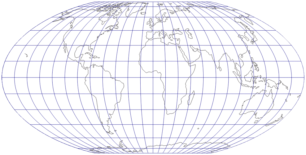
Hufnagel Map Projection Images

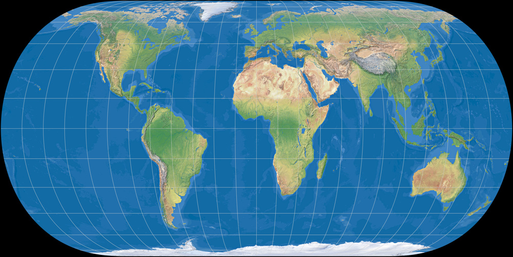
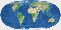
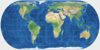
Hufnagel 2

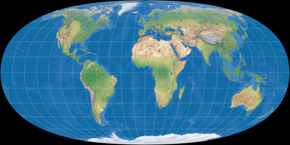
At first glance, Hufnagel 2 seems very similar to the Tobler hyperelliptical projection – but in direct comparison the differences become more obvious:
Hufnagel 2 vs. Tobler hyperelliptical projection

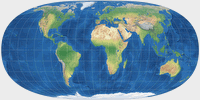
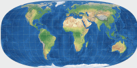
The projections 3 and 4 are very close to No. 2 (and thus, close to Tobler), but show, according to Hufnagel »progressively better distortion values« – which is supported by Capek’s distortion characterization: While on Hufnagel 2, Q is 75.8; Hufnagel 3 has Q = 76.7 and the fourth projection is being noted with a value of 77.8.

Hufnagel 3

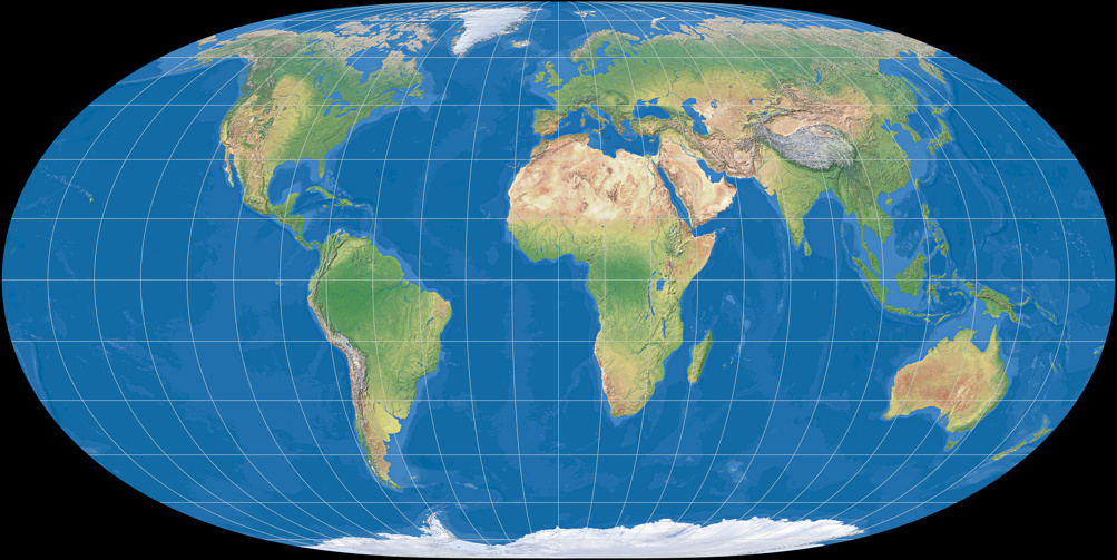
Hufnagel 4

Being very similar projections, the direct comparison might be helpful:
Hufnagel 2 vs. Hufnagel 3
Hufnagel 3 vs. Hufnagel 4
Hufnagel 2 vs. Hufnagel 4

By the way, in his 1989 article Hufnagel mentions that he already published a projection in 1974 – and from the context, I'm inclined to assume that it might have been of of the three projections mentioned above.
However, I don’t know, so if anyone knows more about this, please drop me a line!

 

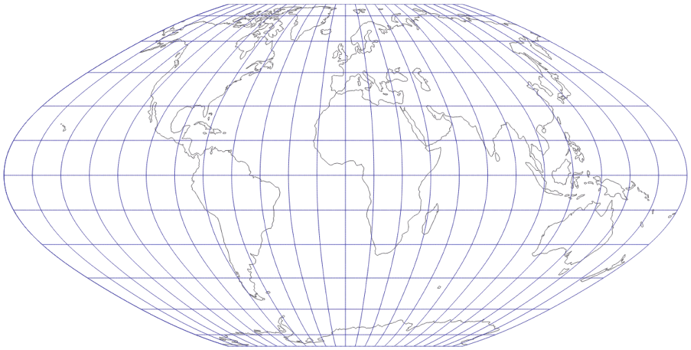
The following three projections present a pole line – and again, progressively decreasing distortions.

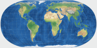
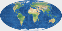
Hufnagel 7

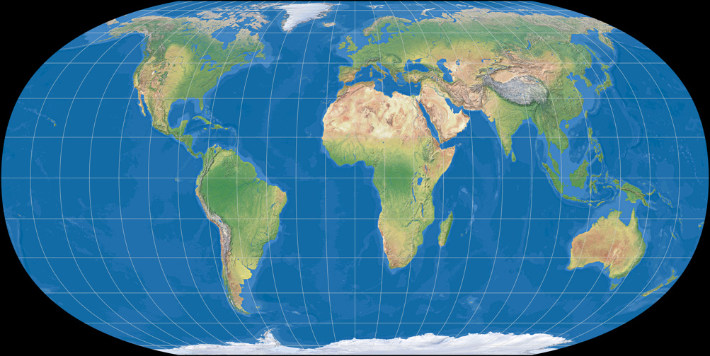
Hufnagel 7 has Q = 79.7; in contrast to No. 9 and 10 the corners aren’t rounded but pointed – which makes Hufnagel 7 my favorite among these three projections, I seem to be a »pointed-corner« kind of guy. ;-)

Looking at Hufnagel 9 and 10, everyone who’s into map projections might think: »Hey, that looks kinda familiar to me…«

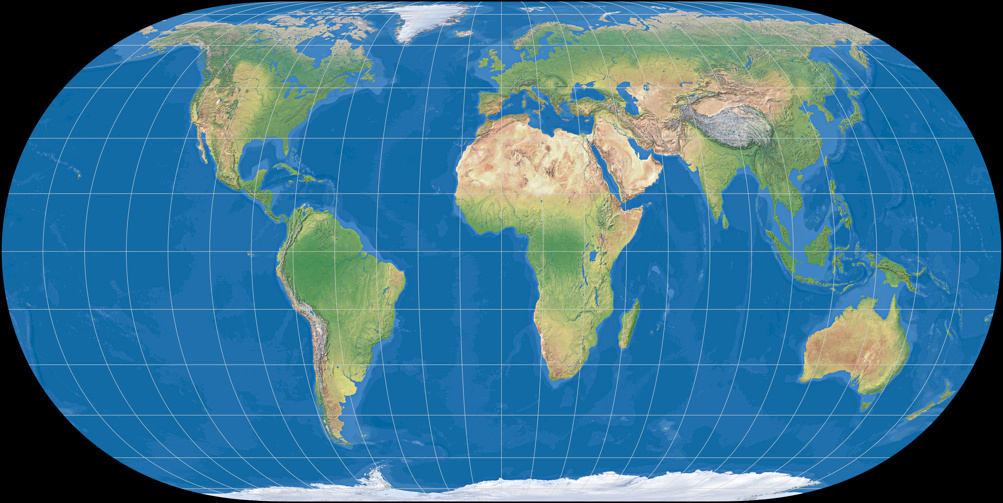
Hufnagel 9

Hufnagel 10

Both are quite alike to the well-known Eckert IV, especially Hufnagel 9:
Hufnagel 9 vs. Eckert IV

No. 10 shows better distortions values (Q = 83.2 vs. Q = 80.1 on No. 9), nonetheless Mr. Hufnagel describes the ninth projection as »aesthetically best balanced« among his projections with a pole line. While I agree that Hufnagel 9 looks more beautiful to me than 10, I do think that Hufnagel 10 is a more valueable addition to the realm of map projections:
Firstly because of its better distortion values, secondly because… well, Hufnagel 9 is awfully close to Eckert IV, appearing more like a variation of the well-known projection, while Hufnagel 10 is much more distinct.
Hufnagel 9 vs. Hufnagel 10

 

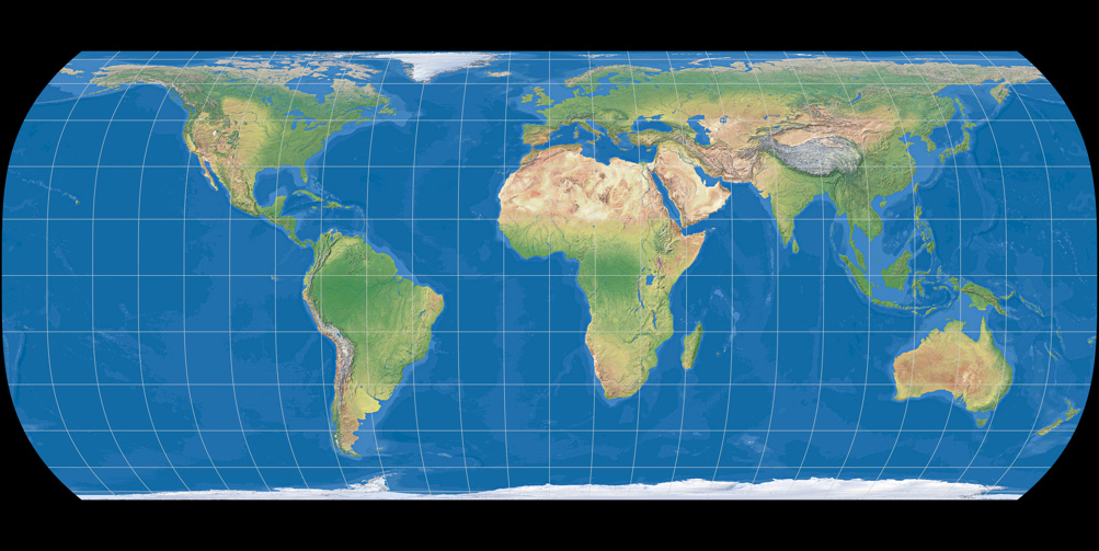
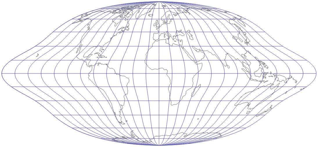
On the next projection, Hufnagel chooses to return to a design where poles are points:

Hufnagel 11

The most distinctive feature are the meridians which aren’t curved but flat around the equator.
Capek notes Hufnagel 11 with Q = 78.3 and thus, the best distortion values among Hufnagel’s pointed pole projections. Hufnagel himself describes the shape of this projection as »takes some getting used to, to say the least« – and who am I to disagree with the creator? ;-)

Nonetheless I kind of like the Hufnagel 11, precisely because it’s quite distinctive.
In marked contrast to Hufnagel’s series of projections:

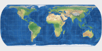
Hufnagel 12

We know that, don’t we?
Hufnagel 12 is a declared variation of the Behrmann projection (Q = 79.7 – unfortunately, Capek doesn’t state Behrmann’s Q value). And since Hufnagel himself doubts the practical use of this projection, I don’t feel compelled to say more about it.
Hufnagel 12 vs. Behrmann

 

The Formulæ

I know: If I introduce the Hufnagel projections, I should add the formulæ to generate them. But there are people who can do this better than me – you can read the formulæ in a publication by Bernhard Jenny, Bojan Šavrič and Daniel »daan« Strebe. ^[3]

However, there are a few things that I’d like to say about this now: Strictly speaking, there are no Hufnagel formulæ (plural) but a single Hufnagel formula (singular): The eight projections Hufnagel presented are generated by assigning appropriate values to four certain variables that Hufnagel called A, B and Ψ_max, additionally you can set the equator-to-central-meridian ratio. The resulting projection is always equa-area. And by setting the right values here, you can not only render all Hufnagel projections but also projections that match Mollweide, Eckert IV, Wagner IV and the Cylindrical Equal-Area and approximate Eckert VI.

But see for yourself:
On mapthematics.com/interactive/hufnagel.html you can not only select the Hufnagel projections, but change the afforementioned variables by dragging a slider. This way, you easily can build your own Hufnagel Variations, which might even be usable…

… or loosely resemble the uninterrupted Goode projection… or you can generate an equal-area projection that approximates the outer shape of the popular Winkel Tripel’s (in case you want such a thing, which you probably don’t)…

… but I kind of like the results when you apply a (short) pole line to the Hufnagel 2 – or use a Length Ratio of 2.0 on the Winkel-Tripel-shaped projection shown above…

… or you can build projections that you most likely wouldn’t use but fun to look at.

 
 

While some of the examples above might of course be superfluous, they still prove the flexibility of Hufnagel’s formula, which therefore is a valueable addition to the field of pseudocylindric map projections.

 

Hufnagel Projections – Synopsis Table

	Projection	Q	Dan	A	B	Ψmax	α
	Hufnagel 2	75.80	30.33	0.05556	-0.05556	90°	2
	Hufnagel 3	76.70	30.27	0.5	0.05556	90°	2
	Hufnagel 4	77.80	29.52	0.08333	-0.08333	90°	2
	Hufnagel 7	79.70	28.97	0.08333	-0.08333	60°	2
	Hufnagel 9	80.10	28.80	0.66667	-0.33333	45°	2
	Hufnagel 10	83.20	28.22	-0.66667	0.66667	30°	2
	Hufnagel 11	78.30	28.81	0	-0.11111	90°	2
	Hufnagel 12	79.70	25.79	0	-0.11111	40°	2.44
As mentioned above, you can generate (or, in one case, approximate) a few established projections using the Hufnagel formula. Here are the corresponding values:
	Mollweide	70.60	32.28	0	0	90°	2
	Eckert VI (Approximation)	69.50	32.43	-0.095	0.095	60°	2
	Wagner IV	76.30	30.39	0	0	60°	2
	Eckert IV	81.90	28.73	1	0	45°	2

 

Hufnagel Approximations

For a while I used approximations for some of the Hufnagel projection images. They have been replaced by now. However, you can still read the section about the approximations in the Approximations chapter.

References

1. ↑ Hufnagel, Herbert:
   Ein System unecht-zylindrischer Kartennetze für Erdkarten.
   In: Kartographische Nachrichten 39/3: 89-96; München Juni 1989.
2. ↑ Capek, Richard 2001:
   Which is the Best Projection for the World Map?
   icaci.org/files/documents/ICC_proceedings/ICC2001/icc2001/file/f24014.pdf
3. ↑ Jenny, B., Savric, B. and Strebe, R. D. 2016
   A computational method for the Hufnagel pseudocylindric map projection family
   download at researchgate.net

Back to Selected Projections  •  Go to top